Hidden Markov Model Market Regimes: How HMM Detects Market Regimes in Trading Strategies

What Are Market Regimes in Financial Markets and Why They Matter for Trading

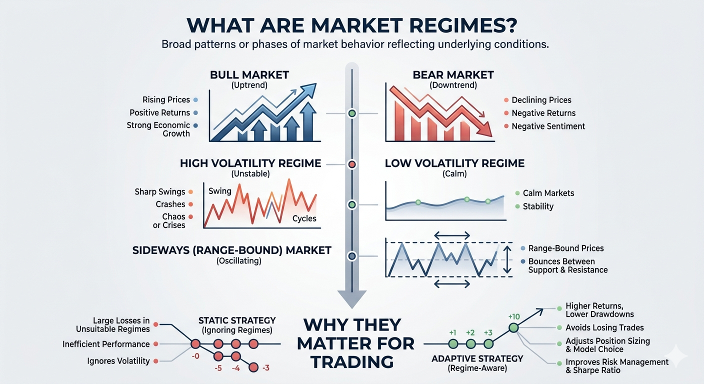
Market regimes are broad patterns or phases of market behavior (for example, periods of high or low volatility) that persist for some time. They reflect underlying macro conditions, investor sentiment, or other factors that cause markets to behave differently over time. For instance, a sustained bull market (rising prices) is a regime, as is a bear market (falling prices), or a quiet low-volatility period. Recognizing regimes matters because many trading strategies assume the market is “stationary,” but real markets switch between calm and chaotic modes. Adapting a strategy when the regime changes can improve risk management and returns.

Common Types of Market Regimes (Bull, Bear, High Volatility, and Sideways Markets)

Common regimes include bull markets (sustained uptrends with positive returns), bear markets (sustained downtrends with negative returns), high-volatility regimes (sharp swings or crashes), low-volatility regimes (calm markets), and sideways (range-bound) markets. A bull market occurs when prices rise persistently, often accompanied by strong economic growth. Conversely, a bear market is defined by declining prices and negative sentiment. In a sideways or non-trending regime, prices oscillate within a relatively tight range. During these lateral phases, supply and demand balance out so that prices bounce between support and resistance levels. Volatility regimes can be thought of separately: a high-volatility regime (often during bear markets or crises) versus low-volatility (typical of sustained bull markets). Since volatility tends to cluster, detecting when it is unusually high or low is also part of regime classification.

Why Market Regime Detection Is Critical for Quantitative Trading Strategies

Identifying regimes lets traders adapt to changing market conditions. A strategy that works well in a bull market may suffer large losses in a volatile bear market, so knowing the regime can prevent unprofitable trades. For example, one study showed that using an HMM to avoid trades in high-volatility regimes eliminated many losing trades and improved the strategy’s Sharpe ratio. In general, regime-aware models can yield higher returns and lower drawdowns. Indeed, research has found that ignoring volatility regimes (i.e. using a static strategy) can hurt performance, whereas adapting allocations based on detected regimes leads to better outcomes. In short, regime detection is critical because it allows quantitative strategies to shift their behavior (positioning, size, or model choice) when the market’s character changes.

What Is a Hidden Markov Model (HMM) in Quantitative Finance?

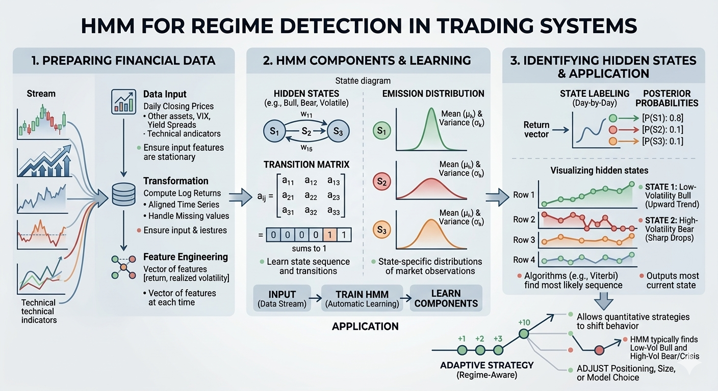
A Hidden Markov Model (HMM) is a statistical state-space model that assumes an underlying, unobserved (“hidden”) state drives the behavior of observed data. In a financial context, we imagine that at each point in time the market is in one of several latent regimes (states) such as “bull,” “bear,” or “sideways.” We can’t observe these states directly, but they influence observable data like returns or volatility. The HMM is memory-less (Markovian), so the next state depends only on the current state. Each hidden state has its own probability distribution for the observable outputs (for example, one state might emit returns with a high positive mean and low variance, and another state with negative mean and high variance). Fitting an HMM to historical market data means we let an algorithm learn the transition probabilities between regimes and the statistical profile of each regime. In practice, this allows us to infer the most likely current market regime from recent data and even estimate probabilities of switching to different regimes.

How Hidden Markov Models Work for Market Regime Detection

To use an HMM for regime detection, we fit the model to historical market data (typically asset returns or related features). The training (usually via the Baum–Welch expectation-maximization algorithm) finds the optimal transition matrix (probabilities of moving from one hidden state to another) and the emission distributions (the statistical profile of returns in each state). After fitting, the HMM can decode the most likely sequence of hidden states that generated the observed data. For each time step, we can compute either the single best state sequence (using the Viterbi algorithm) or the probability of each state given the observations (forward–backward probabilities). In effect, the HMM learns which patterns of returns or volatility characterize each state. For example, an HMM trained on equity index data often finds that one hidden state has a relatively small average return and low volatility (a “normal” or bull regime) and another state has a large negative average return and high volatility (a “crash” or bear regime). Once trained, the model can take new market data and output the most likely current regime or the probabilities of being in each regime, which traders can use to adapt their strategy.

Key Components of a Hidden Markov Model in Trading Systems

An HMM is specified by:

• Hidden states (K): a chosen number of discrete regimes (e.g. 2, 3, 4).
• Transition matrix: a K×K matrix where each entry $a_{ij}$ is the probability of moving from state i to j on the next period. Each row sums to 1.
• Emission (observation) distributions: for each hidden state k, a probability distribution for the observed features. In financial HMMs this is often a Gaussian distribution of returns (with its own mean and variance) for state k.
• Initial state probabilities: the probability of starting in each state at the beginning.

When the HMM is fitted to data, it learns these components automatically. In practice, a fitted Gaussian HMM will give us a transition matrix and state-specific means and variances. For example, one illustrative run from the hmmlearn library printed out a transition matrix along with the mean and variance for each hidden state. In summary, the core components of an HMM in trading are the number of hidden regimes, the matrix of transition probabilities between regimes, and the state-dependent distributions of market observations.

How Hidden Markov Models Identify Hidden Market States in Financial Time Series

After training, the HMM associates each hidden state with a characteristic return distribution. For instance, one state might have a high average return (bullish regime) while another has a negative average (bearish regime). The model also captures how likely it is to stay in the same regime or switch. To identify the regime on a given day, the model uses algorithms like Viterbi to find the most likely hidden state sequence, or computes the posterior probability of each state given the data. In effect, the HMM clusters the time series into segments that exhibit similar behavior. For example, in practice a 2-state Gaussian HMM trained on S&P 500 returns typically finds one “low-volatility bull” state and one “high-volatility bear/crisis” state. Once calibrated, the HMM can be applied day-by-day: it takes the latest return (or feature vector) and outputs the most probable current state or the probability of being in each state. This probabilistic regime labeling lets traders know, for example, that the market is likely in a bullish or bearish state, even though the underlying state isn’t directly observable.

Figure: Visualizing hidden states. The hmmlearn example above splits a stock’s price history into four hidden regimes. Each panel highlights the price points assigned to one hidden state. This kind of plot makes regime changes visible – for instance, one state might capture a quiet upward trend, while another captures sharp drops.

Preparing Financial Market Data for Hidden Markov Model Regime Detection

The input data must be carefully prepared. Typically we start with price series (e.g. daily closing prices) and compute returns, often log returns or percentage changes, since returns are more stationary than prices. If multiple assets or indices are used, align them in time and handle any missing values. Features often include the asset’s daily return, volatility measures (like rolling standard deviation), or other proxies. It’s crucial to ensure the inputs are stationary (so that their distribution does not drift over time); for example, trending technical indicators can be converted into percent-changes or detrended to stabilize them. Some implementations build a richer feature set by including related market data – for example, combining stock index returns with a volatility index (VIX) or yield spreads. The key is that the HMM expects a sequence of observations; common practice is to supply it a vector of features (e.g. [return, realized volatility]) at each time. Finally, it’s important to divide the data into training and testing periods (often with a walk-forward approach) so that the HMM is trained on past data and then evaluated on future data.

Choosing Input Features for an HMM Trading Model (Returns, Volatility, and Indicators)

Effective regime detection often relies on informative features. The most basic input is the asset’s return series. Additionally, volatility measures (like realized volatility or an index such as the VIX) are popular because volatility tends to spike in certain regimes (e.g. crashes). Traders also often use technical indicators that capture momentum and trend: for example, moving averages, RSI (relative strength index), MACD, or Bollinger Bands. These indicators give context about price momentum or mean-reversion tendencies. In fact, one example implementation generated dozens of indicators (RSI, MACD, Bollinger, etc.) to give the HMM information on momentum, volatility, and trends. Other potential features include credit spreads or interest rate yields to capture economic risk appetite. In one recent tutorial, an HMM was trained on a mix of returns, volatility, the VIX, a 50–200-day moving average trend signal, and a 10-year yield. In general, the inputs should be chosen to highlight differences between regimes (e.g. high-volatility vs low-volatility, bullish vs bearish conditions) and should be scaled or normalized if needed. Most HMM implementations (like Gaussian HMMs) assume roughly Gaussian features, so extreme outliers may need special handling (for example by transforming volatility features).

Training a Hidden Markov Model to Detect Market Regimes

Training an HMM involves fitting its parameters to historical data. Practically, one chooses a number of hidden states (see below), initializes the model (e.g. a GaussianHMM in Python’s hmmlearn library), and then calls a .fit() method on the time series. This runs the Baum–Welch (EM) algorithm, which iteratively updates the transition probabilities and emission distributions to maximize the data’s likelihood. In code, training might look like model = GaussianHMM(n_components=K).fit(X), where X is the return series (or feature matrix). It’s important to train on a suitable in-sample period; for example, one backtest trained the HMM on 1993–2004 S&P 500 data and then held it fixed for a 2005–2014 test. In other approaches, the model is retrained periodically using a rolling window of recent data (a “walk-forward” scheme) to adapt to new conditions. When training multiple models with different K, information criteria like the Bayesian Information Criterion (BIC) can help choose the best model: one can fit models with several K (e.g. 2–5 states) and pick the one with lowest BIC. After training, you examine the fitted parameters (transition matrix and state means/variances) to ensure they make sense (e.g. one state should have higher mean return if that’s intended to be a bull regime).

Interpreting Hidden Markov Model Outputs and Regime Probabilities

Once the HMM is fitted, we interpret its output to identify regimes. The primary outputs are:

• The transition matrix (how likely each regime is to follow another),
• The state-specific parameters (for a Gaussian HMM, each hidden state has a mean and variance of returns), and
• The decoded state sequence or probabilities for each time step.

For example, the model might tell us that state 0 has mean return +0.02% and state 1 has mean -0.36%, clearly marking state 0 as bullish and state 1 as bearish in this case. The transition matrix might show high self-transition probabilities, indicating regimes tend to persist. We can use the Viterbi algorithm to label each historical day with the most likely state, or we can compute the probability that the market is in each regime at the current time. In trading, these probabilities often drive decisions. For instance, one strategy uses the HMM to predict the probability of being in a “low-volatility” vs “high-volatility” regime for the next day; then it applies the signal from the model specialized for that regime. In summary, we look at the fitted means/variances to name the regimes (e.g. “bull” vs “bear”), and we use Viterbi or state probabilities to see which regime the market is in or will likely be in.

Visualizing Market Regimes Identified by Hidden Markov Models

To make the regimes interpretable, it’s common to plot them. For example, one can plot the asset price or returns over time and highlight the segments that belong to each hidden state. The hmmlearn tutorial does exactly this: it colors Intel’s stock price by state (each hidden state’s points are plotted in a separate color or subplot). Such charts clearly show the periods classified as each regime. Another approach is to plot the state probabilities over time as colored areas or an additional time series beneath the price chart. These visuals help traders see how the model’s regimes align with known market events (e.g. identifying high-volatility crashes). In practice, seeing the regimes overlaid on the price chart is a powerful diagnostic to ensure the model has learned something meaningful about market behavior.

Building a Hidden Markov Model Trading Strategy Based on Market Regimes

Once market regimes are identified by the HMM, a trader can design strategies that respond to the current regime. A simple approach is to use regime as a trade filter or position modifier. For example, one might pair a basic trend-following strategy (e.g. moving average crossover) with the HMM: allow or enlarge long positions only when the HMM predicts a “bull” regime, and avoid or shrink positions during a “bear” regime. Alternatively, as shown in one example, the HMM can route trading signals to different “expert” models: if the HMM predicts tomorrow will be in Regime 0 (say low-vol), the system uses the model trained on Regime 0 data; if it predicts Regime 1, it uses the other model’s prediction. Another tactic is to use the HMM as a stop-loss trigger: for instance, immediately liquidate or cash out if the model switches to the high-volatility state. In all cases, the HMM output (state or state probability) directly informs the trading rules. In practice, traders often implement this within a backtesting framework: the HMM is trained on historical data, then during each backtest step it classifies the current regime and the strategy uses that label to decide on entries/exits or sizing.

Trend Following Strategies Using Hidden Markov Model Bull Market Regimes

In identified bull-market regimes, one would typically employ trend-following or momentum strategies. For example, if the HMM signals a bullish regime (a hidden state with a positive mean return), the strategy might take long positions on breakouts or buy triggers like a moving-average crossover. In fact, a studied strategy simply went long whenever the 10-day moving average crossed above the 30-day moving average (a bullish signal). When the HMM indicated a bull regime, those long signals were allowed; if the regime was bearish or volatile, trades were skipped. This leverages the fact that trend-following usually performs well in prolonged uptrends. Other trend-based signals (such as momentum oscillators or higher-high price action) could similarly be activated only during the HMM’s bull regimes to improve their hit rate.

Mean Reversion Trading Strategies in Sideways Market Regimes

During a sideways or range-bound regime, mean-reversion strategies tend to work better than trend-following. If the HMM detects a non-trending state, a trader might switch to buying dips and selling rallies within the range. For example, one could buy at identified support levels and sell at resistance, possibly using indicators like RSI or Bollinger Bands to time entries. Investing literature suggests that in sideways markets, traders “profit by taking profits between the support and resistance levels, buying at support and selling at resistance”. Thus, when the HMM labels the regime as sideways (or low volatility with no clear trend), the system would apply such mean-reversion rules. The HMM essentially acts as a regime switch, allocating capital to range-trading models instead of trending models during these periods.

Volatility-Based Position Sizing Using HMM Regime Detection

Hidden Markov models can also inform position sizing based on regime. In a high-volatility regime (as flagged by the HMM), a prudent system might reduce position sizes or leverage to control risk, since prices are swinging unpredictably. Conversely, in a low-volatility regime, it might increase size slightly. For instance, one might set a rule that when the HMM’s predicted regime switches to “high vol,” the strategy cuts risk in half. This is similar to volatility-parity or risk-budgeting ideas, but the novelty is that the regime detector signals when to apply them. Using the HMM this way means the position size dynamically adjusts to the hidden state, potentially smoothing portfolio equity. This approach is especially useful for risk management: it systematically lowers exposure when a turbulent regime is detected, which can reduce drawdowns.

Dynamic Portfolio Allocation Using Hidden Markov Model Market Regimes

Beyond single-asset strategies, HMMs can guide multi-asset or factor allocation. For example, during a bull regime the portfolio might overweight stocks and momentum factors, while in a bear regime it shifts to bonds or defensive factors. Research has demonstrated this: in a factor-investing study, a portfolio that rotated between factor models based on an HMM’s regime predictions significantly outperformed any single factor model alone. In that study, the HMM would identify the regime and choose one of two factor-based portfolios that was best suited to that regime, yielding higher returns overall. More generally, asset allocators can use the HMM state as a macro signal – increasing equity risk on bull signals and raising cash or bonds on bear signals. In practice, a dynamic allocation strategy might have a table of target weights for each regime and switch between them as the HMM transitions.

Backtesting Hidden Markov Model Trading Strategies on Historical Market Data

Backtesting regime-based strategies is essential to evaluate their real-world viability. A common approach is to simulate historical trading with the HMM filter in place. For instance, one backtest trained the HMM on historical S&P 500 data up to year X and then ran a trend strategy from 2005–2014, simply refraining from trades when the model was in the high-volatility state. Another example used a walk-forward backtest on Bitcoin: every day it re-trained the HMM on the most recent 4 years and then applied regime-specific models (see QuantInsti example). The backtest results are then compared to benchmarks (like buy-and-hold). In practice, one plots the equity curves of the HMM-based strategy versus benchmark and computes performance stats. For instance, a recent backtest showed the regime-adaptive strategy (HMM + Random Forest) achieved a higher cumulative return than buy-and-hold, with lower volatility. It is also common to use realistic backtesting methods (no look-ahead bias) such as walk-forward or rolling-window splits. The key is the HMM must only be fit on historical data and then applied out-of-sample. Metrics from these backtests tell us if the regime detection really added value.

Performance Metrics for Evaluating HMM Trading Systems (Sharpe Ratio, Drawdowns, Win Rate)

When evaluating an HMM-based strategy, several metrics are important. The Sharpe Ratio measures risk-adjusted return (mean return divided by volatility). A higher Sharpe means better return per unit of risk. The maximum drawdown captures the worst peak-to-trough loss, reflecting tail risk. The win rate is simply the percentage of trades that were profitable. For example, a backtest of a regime-adaptive strategy reported a Sharpe of about 1.76 versus 1.16 for buy-and-hold, and a smaller maximum drawdown (–20% vs –28%). Other metrics like the Sortino Ratio or Calmar Ratio can also be used. The key is to compare the HMM strategy’s metrics to benchmarks. If the HMM filter or adaptive rules yield a noticeably higher Sharpe or lower drawdown without dramatically reducing return, that indicates a positive impact. It’s also useful to examine the equity curves visually, ensuring that risk is reduced during volatile regimes as intended.

Advantages of Using Hidden Markov Models for Market Regime Detection

HMMs offer several advantages for regime detection. First, they provide a probabilistic, dynamic model of regimes, capturing transitions over time (unlike static clustering). They learn the regimes directly from data without manually defining thresholds. When well-calibrated, HMM-based strategies often improve returns and reduce risk: for instance, studies have found HMM-based allocation “yield superior portfolio results” compared to static approaches and achieve higher returns with lower drawdowns. Another advantage is flexibility: an HMM can be combined with almost any trading rule or machine-learning model, adapting them to regimes. It also naturally accounts for volatility clustering (since high-volatility regimes are separate states). In sum, the main advantage is adaptability – the model can trigger different behavior in bull vs bear conditions in a systematic, data-driven way, which can build “adaptability into its core logic”. Many practitioners find that this state-aware approach improves performance in backtests compared to ignoring regimes.

Limitations and Risks of Hidden Markov Models in Algorithmic Trading

Despite their power, HMMs have limitations and risks. They rely on assumptions that may not hold: for example, a Gaussian HMM assumes normally-distributed returns in each state, which can be wrong during extreme crashes. The Markov property (future depends only on the current state) also ignores longer-term history, which may be important in finance. HMMs are parametric, so mis-specifying the number of states or the type of distribution can hurt. They also can be sensitive to initialization and can converge to local optima. In practice, overfitting is a concern: too many hidden states can make the model chase noise rather than real regimes. Conversely, too few states might lump distinct regimes together. Moreover, the HMM must be trained on historical data, so structural breaks (like new market conditions not seen before) can make it perform poorly out-of-sample. Finally, implementing an HMM adds complexity, and its benefits rely heavily on the quality of input data and features. In short, while HMMs can capture regime shifts, they are not foolproof – their assumptions and parameter choices must be carefully managed.

How to Choose the Optimal Number of Hidden States in an HMM Trading Model

Selecting how many hidden states (K) the HMM should have is an important decision. A common approach is to try several models with different K and compare them using information criteria like the Bayesian Information Criterion (BIC) or Akaike’s AIC. For instance, one practitioner fit HMMs with 3 to 9 states and selected the model with the lowest BIC. In that case, the BIC suggested a surprisingly high K, though practically many traders find that 2–3 states (e.g. bull/bear or bull/neutral/bear) suffice. Domain knowledge can also guide this choice: if you only need to distinguish high-volatility crashes from normal markets, 2 states may be enough. The rule of thumb is to balance complexity: too many states may overfit (capturing noise as “regimes”), while too few may oversimplify and mix different behaviors together. Ultimately, one can validate the choice by checking out-of-sample performance: the best K is the one that yields robust strategy results.

Combining Hidden Markov Models With Technical Indicators and Machine Learning

HMMs are often used in combination with other tools. One approach is to use the HMM’s regime label or probability as an additional feature in another machine-learning model. For example, the QuantInsti tutorial trained a separate Random Forest model for each regime: the HMM first classified each day as “low-vol” or “high-vol,” then two Random Forests were trained on those regime-specific subsets. At run-time, the HMM’s predicted regime decides which model to use for the next signal. Another combo is to use technical indicators both inside the HMM and in parallel trading rules: the HMM might be trained on returns plus a moving-average trend indicator and a volatility indicator, while the actual trading signal might rely on RSI or breakouts. More advanced research even explores hybrids like HMMs feeding into neural networks or reinforcement learners. The key idea is that HMMs can provide the macro regime context, which can enhance the performance of other models. In any case, the HMM does not have to act in isolation; it usually augmentes other signals by gating or modulating them based on regime.

Advanced Applications of Hidden Markov Models in Quantitative Finance

Beyond basic strategies, HMMs have a range of advanced uses. They are applied in factor investing (rotating among factor portfolios as mentioned above), risk allocation (adjusting risk budgets based on regime), and even in option pricing when volatility regimes matter. HMMs can be embedded in volatility models (such as Markov-switching GARCH models) to capture regime-dependent volatility clustering. They have also been used to detect regimes in alternative markets like cryptocurrencies, where volatility shifts are pronounced. In portfolio construction, some research uses HMMs to forecast which factor (value, momentum, etc.) will do best next. HMMs can also feed into machine learning systems (e.g. providing regime signals to a neural network that makes predictions). The “latent states” framework has wide applicability: anytime the market might switch among a few modes (risk-on/off, sector rotations, macro shifts), an HMM can be adapted to model it. In short, HMMs are a flexible tool that can be plugged into many advanced quantitative models, from portfolio optimization to complex signal processing.

Hidden Markov Model vs Other Market Regime Detection Methods

HMMs are one of several regime-detection techniques. A common alternative is static clustering: for instance, one could fit a Gaussian Mixture Model (GMM) or k-means to historical returns and label each period by cluster. Unlike HMMs, these do not consider time dependence – they simply group similar days regardless of sequence. The Two Sigma team, for example, used a GMM on factor returns to identify market “clusters”. More recently, researchers have proposed Wasserstein clustering: they segment the return series into rolling windows, treat each window as an empirical distribution, compute pairwise Wasserstein (Earth-Mover) distances, and then cluster those distributions. This avoids parametric assumptions but does not use Markovian transitions. Traditional econometric methods include regime-switching models (like Hamilton’s Markov-switching model) or threshold-based rules (e.g. if volatility index > X then “high-vol” regime). HMMs sit in the middle: they provide probabilistic state estimates and account for sequence, unlike static clustering. In practice, HMMs often outperform simple threshold rules because they use full distributional information, though more complex methods (e.g. deep learning) are also being explored. The choice often comes down to the data: if market regimes are truly temporally dependent, HMMs capture that; if not, a clustering method might suffice.

Python Implementation of Hidden Markov Models for Market Regime Detection

In Python, popular libraries for HMMs include hmmlearn and pomegranate. The hmmlearn library provides classes like GaussianHMM which can be easily fitted to financial data. In fact, the hmmlearn documentation includes a complete example of fitting a 4-state Gaussian HMM to Intel’s historical stock data, printing out the transition matrix and the mean/variance of each state. Implementing a trading model typically involves: fetching data (e.g. using yfinance or pandas_datareader), computing returns, and then feeding the return series into GaussianHMM(n_components=K).fit(...). One then uses model.predict() or model.predict_proba() to get the hidden states. Many quant traders integrate this into backtesting frameworks like Backtrader or a custom Python loop. Additional tools, such as scikit-learn’s preprocessing or pandas for data handling, are also commonly used. Overall, the Python ecosystem makes it fairly straightforward to implement an HMM: one simply needs to prepare the data and call the library functions as shown in tutorials.

Real-Time Market Regime Detection Using Hidden Markov Models

For live or real-time trading, an HMM can be applied in a streaming fashion. One approach is to fit the HMM on recent history and then, at each new time step, update the probability of each state using the new observation. In practice, some implementations train a static HMM on a historical window and then continually apply it to streaming data: each day’s return is fed into model.predict to get the current state without re-training. This yields a real-time regime label or probability. Other schemes might periodically retrain the HMM (e.g. monthly) to adapt. Because HMMs are probabilistic, they naturally provide a forward-looking regime probability which can be updated on each new tick. This makes them suitable for real-time detection. Of course, any real-time system must carefully avoid look-ahead bias: the HMM must only see past data at any point. When done properly, one can generate live signals like “we are now in Regime 1 with 80% confidence” and act on them immediately. The Python tools above (hmmlearn, etc.) allow incremental prediction on new data, so a real-time pipeline might simply call model.predict as new price data arrive.

Frequently Asked Questions About Hidden Markov Model Trading Strategies

• What is a market regime? A market regime is a broad characterization of market behavior, such as high volatility versus low volatility. It’s essentially a “state” of the market. In this framework, we use an HMM to detect these regimes dynamically. For example, “Regime 0” might represent calm, low-volatility markets, while “Regime 1” is turbulent, high-volatility markets.
• Why train separate models for different regimes? Because a one-size-fits-all model often underperforms. Market dynamics differ by regime, so a model trained only on bull-market data may misbehave in a bear market. Training regime-specific models lets each model specialize. As one author notes, a model trained on specific market conditions “might be better at capturing behavior patterns relevant to that regime” than a single model trained on all data.
• What kind of data does this strategy use? Typically price data (e.g. historical price series from Yahoo Finance) and derived features. Common features include daily returns and technical indicators like RSI, MACD, Bollinger Bands (which capture momentum, volatility, trends). The HMM often takes in returns and any engineered features. In our example, we used daily returns and a variety of technical indicators as inputs for the regime model.
• What machine learning models are used? The core regime detection is done with an HMM, which classifies each period into a hidden state. On top of that, one can use classifiers or regressors to make trading decisions. In one framework, the HMM classifies regimes and then two Random Forest classifiers (one per regime) make predictions about the next move. In general, HMMs and tree/ensemble models are a common combination.
• What’s “walk-forward” backtesting? Walk-forward testing is a method where you repeatedly retrain your models on an expanding window of historical data and then test on the next period. This simulates live trading more realistically. In our context, the HMM (and any associated models) are retrained periodically on past data before being applied to new data, which prevents look-ahead bias.

Conclusion: Using Hidden Markov Models to Improve Market Regime-Based Trading

Hidden Markov Models provide a structured way to detect and exploit market regimes. By modeling the market as a sequence of latent states, an HMM can signal when the market has switched from one regime to another. Traders can use these signals to adapt their strategies—using trend-following models in bull regimes, mean-reversion in sideways regimes, and tightening risk controls in high-vol regimes. The literature shows that regime-adaptive approaches can improve performance: an HMM-driven allocation, for example, produced superior returns compared to any single static strategy. Importantly, this adaptability “builds adaptability into its core logic”, allowing different models or position sizes to be used in each detected regime. Of course, HMMs have limitations (see above), so they should be implemented and validated carefully. But when used judiciously – combined with thoughtful feature engineering, robust backtesting, and risk management – HMMs can be a powerful tool for quantitative traders looking to thrive in shifting market conditions.

Sources: We have cited academic research and industry examples throughout (see citations). Key references include research on regime-switching and factor investing, practical tutorials on HMMs in Python, and empirical analyses of regime-based trading. All facts and figures above are drawn from these vetted sources.