How to Backtest a Trading Strategy

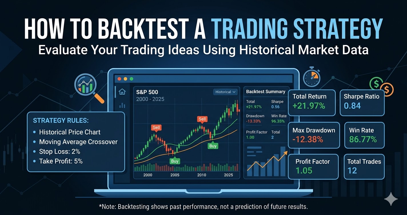
Backtesting means applying a set of trading rules to historical market data to estimate how those rules would have performed in the past. Think of it as a flight simulator for traders. Instead of risking real capital on an untested idea, you run your strategy through years of price data to see what would have happened.

For example, testing a strategy on S&P 500 data from 2000 to 2025 exposes it to the dot-com bust, the 2008 Global Financial Crisis, the 2020 COVID crash, and the post-2022 inflation volatility. This range of market conditions reveals how your trading system behaves when markets boom, crash, or drift sideways.

This article explains how to backtest a trading strategy step by step, covering what data and performance metrics to use and how to avoid common errors. No specific backtesting platform or coding language is required. The focus remains on principles that apply whether you prefer manual backtesting with a spreadsheet or automated backtesting with generic software.

One critical point upfront: backtesting does not predict future performance. Markets change, and past price movements are no guarantee of what comes next. What backtesting does offer is insight into potential risks, returns, and the strategy’s behaviour across different market regimes. It helps you understand your trading strategy’s potential before you commit capital.

By the end of this guide, you will have a practical checklist to backtest your own strategy, whether you trade equities, forex, or other asset classes.

Why backtesting is important for traders

Professional traders at quantitative firms rarely deploy a new idea without first examining how it would have behaved historically. Even experienced discretionary traders benefit from testing their intuitions against past data. The goal is to separate robust trading strategies from random luck.

Testing an equity strategy from 2008 to 2025, for instance, exposes it to multiple recessions, bull markets, and volatility spikes. This long sample helps distinguish genuine edge from strategies that happened to work during one favourable period.

Backtesting also enforces disciplined, rules-based trading. When you see quantitative data showing your strategy’s wins and losses over thousands of trades executed, you replace gut-feeling decisions with objective analysis. This matters when financial markets turn volatile and emotions run high.

Key benefits include:

• Improved precision of entry and exit points
• Better risk management through realistic worst-case scenarios
• More accurate expectations about returns and drawdowns
• Greater confidence to stick with rules during inevitable losing streaks

Backtesting is a research tool, not a guarantee of profit. It must be combined with proper position sizing and risk management tools.

Greater precision in entries and exits

Testing specific trading rules on historical data shows exactly how often signals were profitable. Consider a simple trend-following rule: buy when the 50-day moving average crosses above the 200-day moving average, and sell on the reverse.

Running this rule on daily data for a major index over fifteen years might reveal a 45% win rate. But adding a filter, such as requiring at least a 2% price move after the crossover before entering, could boost that win rate to 52% while cutting the maximum drawdown from 30% to 22%.

Small refinements to your trading logic can make meaningful differences. Adjusting stop-loss distance from 5% to 8% might improve the risk-reward profile from 1:1.5 to 1:2.3 over a decade of testing. These details only become visible when you backtest systematically rather than relying on memory or impressions.

The point is not to chase perfect parameters but to understand which rule variations hold up across different periods and which ones are fragile.

Objective strategy evaluation

Backtesting forces you to define rules clearly. Instead of thinking “this setup usually works,” you specify exactly what triggers an entry, where the stop goes, and when to exit. Two traders following the same written rules should generate identical trade lists.

This clarity transforms vague impressions into measurable statistics: win rate, average profit per trade, profit factor, and maximum drawdown. You can compare how a strategy performed during the 2010–2014 bull market versus the choppier 2015–2020 period.

A strategy that returned 12% annualised with a 15% drawdown during easy conditions but only 8% with a 28% drawdown during mixed conditions reveals its sensitivity to market volatility. This kind of scenario analysis helps you decide whether to discard, modify, or keep a strategy before risking real capital.

Objective evaluation replaces guesswork with quantifiable evidence.

Improved risk management and confidence

Backtesting reveals the worst historical losing streaks and the largest percentage drop from peak equity. Knowing that a strategy experienced a 25% maximum drawdown during 2022 rate-hike volatility helps you size positions realistically.

If your risk tolerance caps drawdowns at 15%, you might allocate only a portion of capital to a strategy with a 25% historical drawdown, or tighten position sizing to 1% account risk per trade. A conservative investor might avoid the strategy entirely, while an aggressive trader might accept the downside risk.

Seeing a strategy survive turbulent periods like March 2020’s 34% market plunge builds genuine confidence. When a new drawdown occurs, you understand it falls within historical norms rather than signalling failure.

Confidence comes from understanding both strengths and weaknesses. A strategy with high returns but enormous swings may not suit your temperament, even if the numbers look attractive on paper.

Prerequisites before you backtest a strategy

Careful preparation determines whether your backtest produces meaningful insights or misleading results. Skipping these steps is the most common reason traders draw false conclusions from their tests.

The key prerequisites are:

• Clear, unambiguous trading rules
• Choice of market, instruments, and time horizon
• Suitable historical period covering multiple market regimes
• Clean, high quality data adjusted for corporate actions
• Basic record-keeping tools (spreadsheet or similar)

Keep preparation practical. For a swing strategy on large-cap US stocks between 2010 and 2025, specify exactly which instruments you would trade, what signals trigger entries, and how you handle exits.

Define a precise trading hypothesis

A trading hypothesis might be: “Buy when the 50-day average crosses above the 200-day average at the prior day’s close, enter at the next day’s open, and exit when the reverse crossover occurs or a 10% stop-loss is hit. Risk 1% of capital per trade, with a maximum of three open positions.”

Every element must be specific enough that two independent traders could implement the same rules and generate identical results.

For a mean-reversion forex strategy, the hypothesis might be: “Short EURUSD when the 14-period RSI exceeds 70 on hourly data, cover when RSI drops below 30 or a 5% stop is triggered.”

Vague rules like “buy when the chart looks bullish” fail the testability requirement. If you cannot write down exact conditions for entry, exit, stop-loss, take-profit, and position sizing, refine your hypothesis before testing.

Choose market, instruments, and time horizon

Markets differ significantly in volatility and behaviour. A strategy designed for large-cap equities will behave differently on cryptocurrency or thinly traded small-caps. Your backtest universe must match your intended live trading universe.

Different strategies require different time horizons:

Strategy Type	Suggested Test Period	Data Resolution
Intraday	6–24 months	Minute or hourly
Swing trading	10–15 years	Daily
Position trading	15–25 years	Daily or weekly

The test period should include multiple phases: bull markets (2010–2019), bear markets (2008, 2022), high volatility (2020 pandemic), and low volatility (2017). Avoid testing only on recent calm periods like 2023–2025, as this can overstate robustness by 20–50%.

Obtain clean and relevant historical data

Your market data should include open, high, low, close prices and, where relevant, volume. For equities, data must be adjusted for stock splits, dividends, and corporate actions.

Poor quality data creates misleading results. Missing prices, erroneous spikes, or unadjusted series can distort backtests significantly. Before testing, run basic sanity checks: look for unusual gaps, verify that major market events appear correctly, and confirm that price movements align with known historical events.

If you choose poor quality data or choose historical data that excludes delisted companies, you introduce survivorship bias that can overstate returns by 2–4% annually.

Work with a reliable data vendor that covers all instruments you intend to trade. Including delisted names where possible reduces survivorship bias. The specified data field requirements depend on your strategy—some need only daily closes, while others require intraday precision.

Step-by-step: how to backtest a trading strategy

This section provides the core backtesting process, laid out as an ordered sequence you can follow with your own rules and data. These steps apply to both manual backtesting and automated backtesting with software.

The main stages are:

1. Formalise rules, assumptions, and costs
2. Apply the strategy to historical data bar by bar
3. Record every trade and build an equity curve
4. Analyse performance with key metrics
5. Refine, re-test, and decide

Visual aids like equity curve charts help interpretation, but the principles remain the same regardless of your tools.

Step 1: Formalise rules, assumptions, and costs

Lock down every aspect of your strategy before touching data. This includes:

• Signal conditions (what triggers entry and exit)
• Position sizing (for example, risk 1% of account per trade)
• Maximum number of concurrent positions
• Stop-loss and take-profit levels

Equally important are realistic assumptions for trading costs. Transaction costs, bid-ask spread, and slippage can significantly reduce apparent profitability.

A practical assumption for large-cap shares might be: 0.01% commission per trade plus 0.05% slippage on entries and exits. For less liquid instruments or intraday trading, increase these figures.

Record all assumptions upfront and keep them consistent across tests. If you compare two strategies tested with different cost assumptions, the comparison is meaningless.

Step 2: Apply the strategy to historical data

Walk forward through the data bar by bar—day by day for daily strategies, hour by hour for intraday. At each bar, check whether entry or exit conditions are met using only information available at that moment.

This prevents look-ahead bias, where you accidentally use future prices to make past decisions.

Example trade walkthrough:

On January 5th, 2015, the 50-day MA crosses above the 200-day MA at the close. Your rules specify buying at the next day’s open. On January 6th, the market opens at 200. You record a hypothetical buy order filled at 200.

The position remains open until March 10th, when the reverse crossover triggers an exit. The market opens at 210, and you record the exit. The gross gain is 5%, which becomes approximately 4.9% after applying your assumed trading costs.

Repeat this process for every signal across your entire backtesting period.

Step 3: Record trades and build an equity curve

Log every trade with these fields:

Field	Description
Date	Entry and exit dates
Instrument	Symbol traded
Direction	Long or short
Entry price	Fill price at entry
Exit price	Fill price at exit
Position size	Units or dollar amount
P&L	Profit or loss after costs
Notes	Relevant context

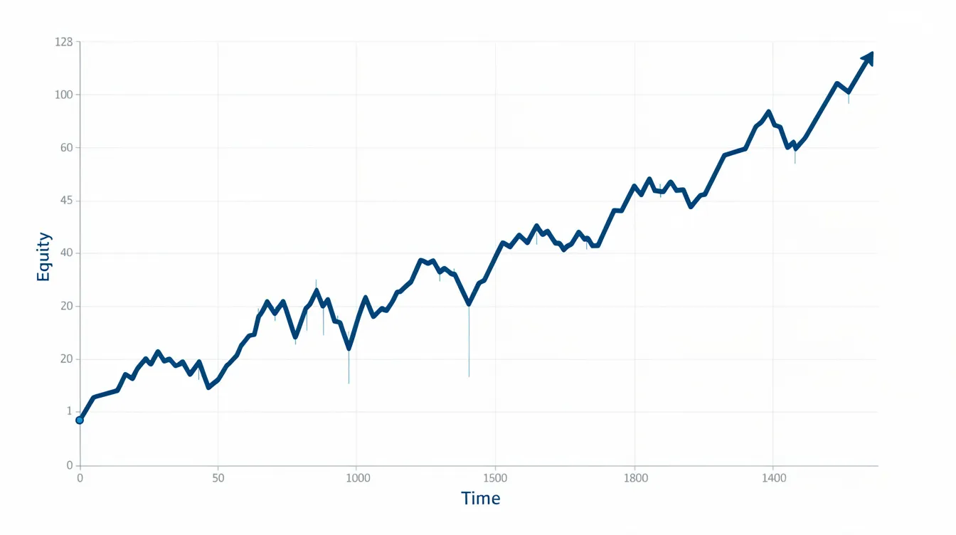
From this log, compute cumulative profit and loss over time to form an equity curve. This curve visually shows growth, drawdowns, and flat periods.

A trading journal like this makes patterns visible. You might notice that losing trades cluster during specific market conditions or that winning trades share common characteristics.

Step 4: Analyse performance with key metrics

After building the equity curve, compute summary statistics. From January 2010 to December 2025, a hypothetical strategy might show:

• Total return: 80%
• Annualised return (CAGR): 6.2%
• Volatility (monthly): 12%
• Maximum drawdown: 22%
• Sharpe ratio: 0.52
• Win rate: 48%
• Average win: 4.2%
• Average loss: 2.1%
• Profit factor: 1.8

These performance metrics must be interpreted in context. A 6.2% annualised return with a 22% maximum drawdown suits moderate risk tolerance but may be unacceptable for conservative investors expecting smaller swings.

Risk adjusted returns matter more than raw profit. A strategy returning 15% with 40% drawdowns may be less attractive than one returning 8% with 15% drawdowns.

Step 5: Refine, re-test, and decide

Based on observed weaknesses, you might adjust strategy parameters. Perhaps the moving average lengths could be shortened, or the stop-loss widened.

However, making too many small changes to fit one dataset leads to overfitting. The strategy performs beautifully on in sample data but fails on out of sample data.

The solution is out-of-sample validation. Optimise on 2010–2016 data, then test the refined strategy on 2017–2025. If in-sample performance shows a Sharpe ratio of 1.2 but out-of-sample drops to 0.4, the strategy is likely overfit.

Decision framework:

• Discard if profit factor is below 1.2 or drawdown exceeds 30%
• Continue iterating if profit factor is 1.2–1.5
• Advance to paper trading if profit factor exceeds 1.5 with stable out-of-sample performance

Expect several rounds of testing before a strategy is robust enough for forward testing.

Manual vs rules-based (automated) backtesting

Manual backtesting means stepping through historical charts by hand, recording trades in a notebook or spreadsheet. Rules-based backtesting uses software to apply defined rules automatically across datasets.

Both approaches rely on identical underlying trading logic. The difference lies in speed, scale, and potential for human bias.

A trader might manually test three months of hourly data for a forex strategy, scrolling through charts and noting each signal. The same trader could run automated backtesting across twenty years of daily data for 500 equity symbols in minutes.

Manual backtesting: strengths and limitations

Manual backtesting involves scrolling through charts, identifying signals visually, and recording trades executed by hand.

Benefits:

• Develops deeper intuition about price action
• Reveals context around signals (news events, patterns)
• Works well for discretionary or visually interpreted strategies

Drawbacks:

• Time-consuming (perhaps 100 trades per hour maximum)
• Prone to cherry-picking and hindsight bias
• Impractical for testing many variations or long histories

If you manually backtest, you might unconsciously skip trades that looked like losers with hindsight or remember profitable setups more vividly. This bias inflates apparent performance.

Manual backtesting works best for beginners or those with rule-based but visually interpreted strategies, as a first step before scaling up.

Rules-based backtesting: strengths and limitations

Rules-based backtesting uses generic backtesting software to encode exact trade rules and run them across large datasets without human intervention.

Advantages:

• Speed: thousands of trades processed in minutes
• Ability to test multiple instruments and parameter combinations
• Removes emotional bias from signal selection
• Enables strategy tester tool functionality for systematic comparison

Challenges:

• Requires precise rule definition (no ambiguity allowed)
• Risk of building overly complex trading strategies
• Temptation to over-optimise parameters

This approach is a natural evolution for traders who have validated ideas manually and want to scale tests responsibly. Start simple, and add complexity only when justified by robust out-of-sample results.

Selecting tools and data sources for backtesting

Traders need three components for backtesting: historical data, a way to view or manipulate that data, and a method to implement rules.

The specific backtesting platform matters less than data quality and tool reliability. Features to prioritise over brand names include:

• Ability to export or log trades
• Multi-instrument support
• Built-in statistical calculations
• Equity curve visualisation
• Transaction cost and slippage simulation

Start with tools you can understand and maintain. A sophisticated setup that you cannot debug or verify produces less reliable results than a simple spreadsheet you control completely.

Both free backtesting tools and free backtesting software exist for traders starting out, though professional traders often invest in more comprehensive solutions as their strategies mature.

What to look for in historical data and tooling

Desirable data characteristics:

• Long history (15+ years for position strategies)
• Coverage of different market regimes
• Corporate action adjustments (splits, dividends)
• Accurate timestamps for intraday strategies

Useful tool features:

• Trade logging and export capability
• Handling of multiple instruments and different asset classes
• Basic statistics calculation
• Visual performance charts
• Customisable cost assumptions

Ensure your chosen backtesting software or trading platform can easily incorporate transaction costs and slippage. A strategy that looks profitable with zero costs may become unprofitable once realistic expenses are applied.

Key performance metrics in backtesting

Raw profit alone tells an incomplete story. You must understand risk, variability, and the path of returns to judge whether a strategy suits your objectives.

These metrics translate backtesting results into actionable decisions about position sizing, risk tolerance, and whether to proceed to simulated trading.

Return and risk metrics

Total return shows overall growth. If you started with $10,000 and ended with $18,000 over ten years, your total return is 80%.

Annualised return (CAGR) standardises this for comparison. That 80% over ten years equals approximately 6% annualised. This matters when comparing strategies tested over different periods.

Volatility measures typical fluctuation of returns. Higher volatility means a bumpier equity curve with larger swings. A 12% monthly volatility implies significant ups and downs even if the long-term trend is positive.

Maximum drawdown is the largest peak-to-trough decline in account value. Many traders consider this the single most important risk number. A 25% drawdown means your account fell from its high point to 25% below that level before recovering.

Risk-adjusted performance and trade-level statistics

Risk-adjusted performance answers: “How much return did you earn per unit of risk taken?”

Two strategies might both return 10% annually. If one experienced a 15% maximum drawdown while the other suffered 35%, their attractiveness differs dramatically.

The Sharpe ratio (return divided by volatility, adjusted for risk-free rate) is the most common risk-adjusted measure. Values above 1.0 are generally considered good; above 1.5 is excellent.

Trade-level statistics reveal the strategy’s character:

Metric	What It Tells You
Win rate	Percentage of winning trades
Average win	Mean profit on profitable trades
Average loss	Mean loss on unprofitable trades
Profit factor	Gross profit divided by gross loss

A 55% win rate with small average wins trades differently than a 35% win rate with large average wins. The latter requires psychological tolerance for frequent losing trades before occasional home runs.

Common mistakes and biases in backtesting

Misleading backtests often come from subtle errors rather than obvious ones. Backtesting relies on accurate simulation, but several pitfalls can invalidate results entirely.

The main dangers are:

• Overfitting and over-optimisation
• Look-ahead bias
• Survivorship bias
• Ignoring trading costs
• Unrealistic liquidity assumptions

Avoiding these issues is as important as the strategy rules themselves.

Overfitting and over-optimisation

Overfitting occurs when a strategy is tuned so closely to one historical sample that it captures noise rather than repeatable patterns.

Warning signs:

• Too many adjustable parameters
• Very specific rules that only work on one instrument or period
• Dramatic performance differences outside the optimisation window

For example, you might discover that a 47-day moving average produced optimal results from 2012–2019. But this parameter may simply fit the characteristics of that particular bull market. Testing on 2020–2025 reveals the strategy fails entirely.

Defences:

• Limit adjustable parameters to fewer than five
• Use broad parameter ranges rather than precise values
• Always validate on separate time periods

A slightly less profitable but stable strategy beats a fragile “perfect” historical performer every time.

Look-ahead, survivorship, and cost neglect

Look-ahead bias means using future data to make past decisions. If your rules check the day’s closing price before that day has actually closed, you have introduced look-ahead bias.

Survivorship bias tests only on instruments that still exist today. When you ignore companies that merged, delisted, or failed, you overstate returns by 2–4% annually. The survivors naturally look better than the full universe.

Cost neglect turns apparently profitable strategies into losers. A strategy generating 2% gross returns per month looks attractive until you apply 0.2% round-trip costs on frequent trades.

Safeguards:

• Use only information visible at the time of each decision
• Include delisted instruments in your data where possible
• Stress-test results by increasing assumed costs by 50%

From backtest to forward test: what to do after a promising result

Even a well-conducted backtest is only one stage in evaluation. The next step is forward performance testing, also called paper trading: applying the same rules to current market data in real time without risking real capital.

A phased approach works best:

1. Initial backtest on in-sample data
2. Validation on out-of-sample data
3. Paper trading in a demo account (3–6 months or 50+ trades)
4. Small live allocation (1% of capital)
5. Gradual scaling as confidence builds

Monitor whether paper or live results stay within the range set by the backtest. If drawdowns exceed 1.5x historical levels, something may have changed.

Practical checklist for going from test to live

Before moving from backtest to live trading, confirm:

• [ ] Rules are explicit and unambiguous
• [ ] Transaction costs are realistic (or conservatively high)
• [ ] Test period includes multiple market regimes (GFC, COVID, rate hikes)
• [ ] Out-of-sample validation shows consistent performance
• [ ] Maximum drawdown is acceptable for your risk tolerance
• [ ] Forward testing period covers adequate trades (50+ or several full cycles)

Track forward-test real trades with the same logging system used for backtesting. This enables direct comparison of statistics and reveals whether the strategy performs as expected under future market conditions.

Periodic re-backtesting—annually, at minimum—keeps strategies aligned with evolving markets. The patterns that worked in 2015 may weaken as algorithmic trading and market structure shift.

Conclusion

Effective backtesting combines clear trading rules, high quality data, realistic assumptions about costs, and disciplined interpretation of results. When done properly, the backtesting process helps you gain insights into how your strategy might behave across different market conditions.

Backtesting is a decision-support tool. It narrows the field to trading strategies worth deeper investigation but cannot guarantee future profits in live trading. The equity curve you see in testing reflects past data, not a promise about what comes next.

Start with a simple, well-defined strategy. Test it over a meaningful period—2008 to 2025, for example—to expose it to multiple market regimes. Refine based on out-of-sample results, then move to paper trading before risking real capital. Seek professional advice if you are unsure about specific aspects of your approach.

Markets evolve continuously. Quantitative data from five years ago may no longer represent current conditions. Treat backtesting as an ongoing practice rather than a one-time exercise. Regular re-evaluation keeps your edge aligned with how financial markets actually behave today.